AIデータセンターの800V化：GaNとSiCの違いを電力損失から読む

800V化の話で私が確かめたいのは、どの材料が勝つかより、電力経路のどこから損失が消え、どこに新しい部品が必要になるかだ。GaNとSiCを同じ「AI電源向け半導体」として並べるだけでは、配電、降圧、故障遮断という異なる仕事が見えなくなる。

先に答えを書く。800Vは主に電力を運ぶ側の電圧であり、GPUの動作電圧ではない。 高耐圧側の変換・保護にはSiCを使う設計があり、ラック内の高密度な降圧にはGaNを使う設計がある。ただし役割は材料名だけで固定されない。耐圧、回路方式、負荷、熱、コスト、認証を揃えて比較する必要がある。

AI電力ボトルネックの投資地図で扱った系統・構内・チップ周辺のうち、本稿は構内からラックまでに絞る。2026年9月12日までに確認した一次資料と、条件を明示した独自試算を使う。試算は製品の実測値でも市場予測でもない。

800Vにすると何が変わるのか

私はまず、材料の宣伝文句を外して電流の桁を確認する。

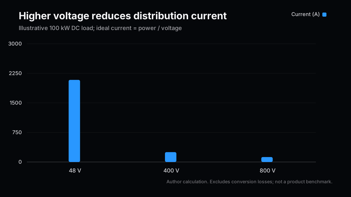
直流の理想化した関係は、電流＝電力÷電圧である。同じ100kWを48Vで運ぶと約2,083A、800Vなら125Aになる。以下は変換損失を無視した電力経路の比較で、特定製品の仕様ではない。

ここで48Vを比較の基準にしたのは、電流差を読み取りやすくするためである。すべての既存ラックが48Vだという意味ではない。TIの技術資料も800Vへの移行と、その先に残る低電圧側の電源を分けて論じている。実際の設備を評価するときは、その設備のバス電圧に置き換える。

配線損失の削減率を設備全体に広げない

同じ抵抗なら配線の発熱は電流の二乗に比例する。800Vと48Vの電流比は0.06なので、配線損失の比は0.0036になる。言い換えると、同じ抵抗・同じ電力という限定条件では99.64%の低下である。しかし、この数字をデータセンターの消費電力削減率として使うのは誤りだ。

実装では導体を細くすれば抵抗が増える。コネクター、保護素子、変換回路にも損失があり、GPU自体の消費電力はこの式から消えない。同じ断面積で損失を減らすのか、損失を一定にして銅を減らすのか、両者を配分するのかで設計は変わる。削減効果を比較する際には、基準となる回路図と測定端子を必ず並べたい。

電流が小さくなっても絶縁設計は容易になるわけではない。800V側を扱う部品には電圧ストレスと過渡条件の評価が必要で、低電圧側の部品をそのまま移せない。配線の省資源化と部品単価の上昇が同時に起きる場合、総コストは両方を積み上げて初めて分かる。

GaNとSiCはどこで使い分けるのか

私の比較単位は、材料そのものではなく「どの変換段を受け持つか」である。

InfineonのIBC資料は800V級の入力から50V、12V、6Vなどの中間電圧へ変換する構成を示している。これは800V化によってラック内のすべてが高電圧に置き換わるわけではないことを示す具体例だ。下表の電圧は機能を整理するための代表値であり、推奨回路でも部品の採用保証でもない。

2026年9月10日付のInfineon日本語発表は、SolarEdgeとの協業でSiC JFETを使う半導体遮断器を扱っている。これは変換効率だけを見ると見落とす部品需要の具体例だ。発表は開発協業を示すもので、採用台数や売上を確定する資料ではない。

「高周波だから有利」の比較条件

スイッチング周波数を上げれば周辺部品を小さくできる余地がある一方、スイッチング損失や駆動、ノイズ、熱の扱いも変わる。ある部品が高周波に適していることと、完成品の効率・価格・信頼性が優れていることは別の検証項目だ。私は効率の最高値より、想定負荷での曲線と温度条件を先に比較したい。

例えばA社が定格負荷時の最高効率を示し、B社が負荷20〜100%の平均を示しているなら、その数字をそのまま横に並べることはできない。入力電圧、出力電圧、出力電力、冷却条件、補助電源を測定に含むかを揃える。同じ「98%」でも測定範囲が違えば意味が変わる。

保護回路も損益計算に入れる

配電経路に常時入る保護素子は、通常運転でも損失に寄与する。効率を高めるために変換段を減らしても、その利得の一部が別の部品で消える可能性がある。一方、故障範囲を小さくできれば停止損失の抑制につながり得る。この便益は電気代とは別の項目で評価したい。

停止時間の価値を計算する場合も、すべてのラックが同時に最大売上を失うという前提を無意識に置かない。冗長化、負荷移動、復旧時間、契約上の扱いを入れる。資料に停止率がなければ、ゼロとも業界平均とも決めず、感度分析の変数として残す。この段階の不確実性が大きいほど、精密に見える投資回収年数は割り引いて読むべきだ。

効率1ポイントを電気代に換算する

ここで私が置く判断軸は、効率の改善幅を年間キャッシュに換算し、導入費用と比較することだ。

出力1MWを一定に保つ変換経路について、入力電力＝出力電力÷効率とする。年間8,760時間、電力単価0.10米ドル/kWhを仮定する。税金、需要料金、冷却設備への波及、故障、導入工事は含めない。効率は全負荷で一定と仮定するため、実施設計には負荷別の測定値が必要だ。

97%から98%への改善は1ポイントだが、入力電力の減少は約10.52kWとなる。この条件で通年稼働すれば約92.15MWh、電気代では約9,215米ドルの差になる。これは「1MWの1%をそのまま使う」近似より、変換経路の境界が明確な計算である。

稼働率で回収額は変わる

実効稼働率を、同じ出力を供給した時間の割合として単純化すると次のようになる。サーバーのCPU利用率やAIモデルの利用率と同義ではない。一定の効率を置いた線形モデルであり、実際の待機電力は別途積み上げる。

追加費用30,000米ドルは計算用の仮定であり、実製品の価格ではない。工事費が上がる、電力単価が下がる、稼働率が低いという条件が重なれば、電気代だけでの回収は長くなる。逆に設置面積の削減や運用の改善が価値を持つ場合もあるが、見積書や実測がない段階で加算しない。

割引率を入れる場合は、毎年の削減額を現在価値に戻してから導入費用と比較する。5年後の同額の節約は今日の支払いと等価ではない。ここでは金利見通しを置かず単純回収だけを示した。案件を評価する際には、想定する設備寿命より回収期間が長くないか、途中交換が必要な部品はないかを先に確かめる。

変換段が複数あるなら効率は掛け合わせる。例えば98%の段が3つなら、経路全体では約94.12%だ。ただし、ある段をなくすと残りの段に要求される変換比や絶縁条件が変わる。段数だけを減らした比較も、個別段の最高効率だけを掛けた比較も、完成品の証明にはならない。比較の出発点として使い、最後は同じ境界で測定する。

ロードマップから売上までの距離を確認する

私が投資判断で慎重になるのは、規格への参加と売上への寄与の間に複数の確認段階があるからだ。

NVIDIAの2026年8月の説明は、既存設備向けのハイブリッド構成と将来の構内全体のDC化を段階として示している。記載された投入予定を、本稿時点の納入実績として読み替えてはいけない。OCPの公開資料も共同仕様と安全面の整合を進める取り組みであり、すべての製品の認証が完了したという意味ではない。

IEAの2026年の更新見通しでは、データセンターの電力消費は2025年の485TWhから2030年に950TWhへ増える想定だ。大きな需要背景ではあるが、その総量に特定材料の取り分を掛ければ企業売上が出るわけではない。配電方式、採用時期、顧客構成、シェア、単価という中間の変数が必要になる。

この表は企業を採点した結果ではなく、資料を読む順番だ。InfineonやTIのように製品群が広い企業では、AI向けの成長があっても他用途の変動に埋もれる可能性がある。特定テーマへの集中が大きい企業では、その反対に採用延期の影響が大きくなり得る。いずれも最新決算の内訳を確認するまでは確定しない。

投資判断は技術と価格を分ける

本稿の技術テーマに対する見方は、短期は採用実績の確認を優先、中期は電源変換と保護を併せて追跡する、である。GaNかSiCかを一つ選ぶ判断にはしていない。企業の現在株価、予想利益、バランスシートを本稿では評価していないため、個別株の割安・割高や売買推奨も結論に含めない。

私なら次の決算で、対象製品の量産時期、顧客評価から受注への転換、供給能力と在庫の動きを同じ表に置く。受注増が在庫増と一緒に進んでいる場合は、その理由も読む。技術的な必要性が高いことと、株主への利益が大きいことの間にある仮定を一つずつ減らすためだ。

2027年までに何を追うか

現時点の私の中心シナリオは、既存設備と新設設備で異なる移行速度が続くというものだ。これは予測確率を付けたモデルではなく、次の資料で更新するための仮説である。

電力不足はラックの電圧を上げるだけでは解消しない。発電や系統接続の容量が増えるわけではないからだ。800V化を評価する理由は、供給された電力をより少ない配線負担と合理的な変換経路で届ける選択肢だからである。この役割を限定するほうが、設備投資のどこを追うべきかがはっきりする。

次回の確認項目は3つに絞る。まず、公式の量産予定が実際の出荷へ進んだか。次に、効率の数字に測定境界と負荷条件が付いているか。最後に、保護機能と保守を含む導入費用が分かるか。この3点が揃えば、材料の優劣という大きな議論を、個別の設備にとって採用する価値があるかという判断に変えられる。

関連記事

• AI電力ボトルネックとパワー半導体の投資地図 — 系統からチップまでの役割を整理する。
• データセンター周辺領域の投資地図 — 電源と冷却・光接続を同じ設備投資の中で比較する。
• メモリとアクセラレータの距離を縮める実装基板 — 電力経路とは別に、信号と実装の制約を読む。

次号の記事案

• 案1：800Vの保護回路を比較する — 半導体遮断器の通常時損失と故障時の挙動を分け、量産採用までの確認事項を整理する。
• 案2：電源効率と稼働率から投資回収を計算する — 同じ設備費でも負荷曲線と電気料金で判断が変わる範囲を検証する。
• 案3：電源メーカーの決算で800V売上を追う — 次の四半期に、開発協業から出荷への進展をどの開示で確認できるかを調べる。

参考資料

• NVIDIA：800V DC電源アーキテクチャの移行段階（2026年8月11日）
• TI：800V DC配電の技術解説（2026年5月改訂）
• Infineon：中間バスコンバーターの構成
• Infineon：SolarEdgeとの800V DC保護技術協業（2026年9月10日）
• Open Compute Project：共同仕様と移行方針（2026年8月11日）
• IEA：Key Questions on Energy and AIの要旨

本記事は情報提供であり投資助言ではありません。筆者が記載企業の株式等を保有している可能性があります。調査・執筆・翻訳に生成AIを利用しています。試算は明示した仮定に基づき、製品性能や投資収益を保証しません。詳細は免責事項をご確認ください。